This tutorial shows how to implement LSTNet, a multivariate time series forecasting model submitted by Wei-Cheng Chang, Yiming Yang, Hanxiao Liu and Guokun Lai in their paper Modeling Long- and Short-Term Temporal Patterns in March 2017. This model achieved state of the art performance on 3 of the 4 public datasets it was evaluated on.
We will use MXNet to train a neural network with convolutional, recurrent, recurrent-skip and autoregressive components. The result is a model that predicts the future value for all input variables, given a specific horizon.
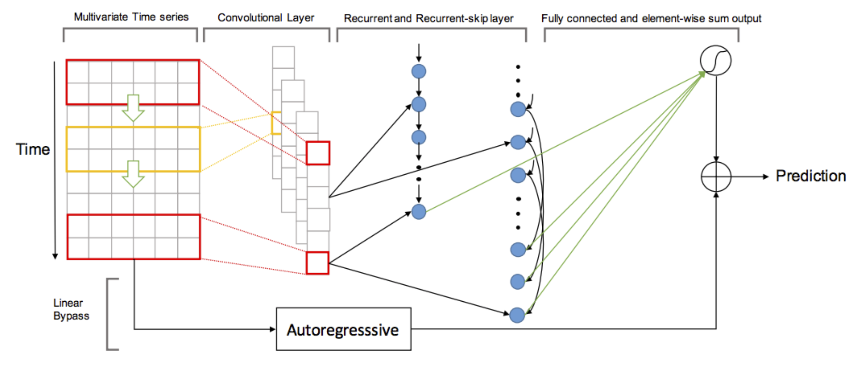
Image from Modeling Long- and Short-Term Temporal Patterns with Deep Neural Networks, Figure 2
Our first step will be to clone the repository and download the public electricity dataset used in the paper. This dataset comprises measurements of electricity consumption in kWh every hour from 2012 to 2014 for 321 different clients.
$ git clone git@github.com:opringle/multivariate_time_series_forecasting.git && cd multivariate_time_series_forecasting
$ mkdir data && cd data
$ wget https://github.com/laiguokun/multivariate-time-series-data/raw/master/electricity/electricity.txt.gz
$ gunzip electricity.txt.gz
Before constructing the network, we need to build data iterators. These will feed batches of features and targets to the module during training. In this network, the target for each example is the value of all time series h steps ahead of the current time. The features for each example are the q previous values, for all time series. In other words, we want to build a model which can predict the electricity consumption of any house h measurements into the future, given the past q electricity consumption readings for all houses.
The following function reads in the electricity time series data, generates examples based on q and h, splits these into training, validation and test sets and returns mx.NDArrayIters to feed the network.
def build_iters(data_dir, max_records, q, horizon, splits, batch_size):
    """
    Load & generate training examples from multivariate time series data
    :return: data iters & variables required to define network architecture
    """
    # Read in data as numpy array
    df = pd.read_csv(os.path.join(data_dir, "electricity.txt"), sep=",", header=None)
    feature_df = df.iloc[:, :].astype(float)
    x = feature_df.as_matrix()
    x = x[:max_records] if max_records else x

    # Construct training examples based on horizon and window
    x_ts = np.zeros((x.shape[0] - q, q, x.shape[1]))
    y_ts = np.zeros((x.shape[0] - q, x.shape[1]))
    for n in range(x.shape[0]):
        if n + 1 < q:
            continue
        elif n + 1 + horizon > x.shape[0]:
            continue
        else:
            y_n = x[n + horizon, :]
            x_n = x[n + 1 - q:n + 1, :]
        x_ts[n-q] = x_n
        y_ts[n-q] = y_n

    # Split into training and testing data
    training_examples = int(x_ts.shape[0] * splits[0])
    valid_examples = int(x_ts.shape[0] * splits[1])
    x_train, y_train = x_ts[:training_examples], \
                       y_ts[:training_examples]
    x_valid, y_valid = x_ts[training_examples:training_examples + valid_examples], \
                       y_ts[training_examples:training_examples + valid_examples]
    x_test, y_test = x_ts[training_examples + valid_examples:], \
                     y_ts[training_examples + valid_examples:]

    #build iterators to feed batches to network
    train_iter = mx.io.NDArrayIter(data=x_train,
                                   label=y_train,
                                   batch_size=batch_size)
    val_iter = mx.io.NDArrayIter(data=x_valid,
                                 label=y_valid,
                                 batch_size=batch_size)
    test_iter = mx.io.NDArrayIter(data=x_test,
                                  label=y_test,
                                  batch_size=batch_size)
    return train_iter, val_iter, test_iter
Time to build the network symbol. This is a graph, which represents the architecture of our neural network. If you’re not solid on convolutional & recurrent layers, check out this blog post on CNNs & this awesome blog post on LSTMs.
First a convolutional layer is used to extract features from the input data. Here, kernels with shape = (number of time series, filter_size) pass over the input. The input is dynamically padded, depending on the height of the kernel. This ensures, as each filter slides over the input data, it produces a 1D array of length q. Dropout is applied to the resulting layer, which has shape = (batch size, q, total number of filters).
These convolutional features are used in two components of the network. The first is a simple recurrent layer. A gated recurrent unit is unrolled through q time steps. Each unrolled cell receives input data of shape = (batch size, total number of filters), along with the output from the previous cell. The output of the last unrolled cell is used later in the network.
The output from the convolutional layer is also passed to the recurrent-skip component. Again a gated recurrent unit is unrolled through q time steps. The outputs from unrolled units a prespecified time interval (seasonal period) apart are used later in the network. In practice recurrent cells do not capture long term dependencies. When predicting electricity consumption the measurements from the previous day could be very useful predictors. By introducing skip connections 24 hours apart we ensure the model can leverage these historical dependencies.
The final component is a simple autoregressive layer. This splits the input data into its 321 individual time series and passes each to a fully connected layer of size 1, with no activation function. The effect of this is to predict the next value as a linear combination of the previous q values.
The sum of the output from the autogressive, recurrent and recurrent-skip components is used to predict the future value for every time series. The L2 loss function is used.
def sym_gen(train_iter, q, filter_list, num_filter, dropout, rcells, skiprcells, seasonal_period, time_interval):

    input_feature_shape = train_iter.provide_data[0][1]
    X = mx.symbol.Variable(train_iter.provide_data[0].name)
    Y = mx.sym.Variable(train_iter.provide_label[0].name)

    # reshape data before applying convolutional layer (takes 4D shape incase you ever work with images)
    conv_input = mx.sym.reshape(data=X, shape=(0, 1, q, -1))

    ###############
    # CNN Component
    ###############
    outputs = []
    for i, filter_size in enumerate(filter_list):
        # pad input array to ensure number output rows = number input rows after applying kernel
        padi = mx.sym.pad(data=conv_input, mode="constant", constant_value=0,
                          pad_width=(0, 0, 0, 0, filter_size - 1, 0, 0, 0))
        convi = mx.sym.Convolution(data=padi, kernel=(filter_size, input_feature_shape[2]), num_filter=num_filter)
        acti = mx.sym.Activation(data=convi, act_type='relu')
        trans = mx.sym.reshape(mx.sym.transpose(data=acti, axes=(0, 2, 1, 3)), shape=(0, 0, 0))
        outputs.append(trans)
    cnn_features = mx.sym.Concat(*outputs, dim=2)
    cnn_reg_features = mx.sym.Dropout(cnn_features, p=dropout)

    ###############
    # RNN Component
    ###############
    stacked_rnn_cells = mx.rnn.SequentialRNNCell()
    for i, recurrent_cell in enumerate(rcells):
        stacked_rnn_cells.add(recurrent_cell)
        stacked_rnn_cells.add(mx.rnn.DropoutCell(dropout))
    outputs, states = stacked_rnn_cells.unroll(length=q, inputs=cnn_reg_features, merge_outputs=False)
    rnn_features = outputs[-1] #only take value from final unrolled cell for use later

    ####################
    # Skip-RNN Component
    ####################
    stacked_rnn_cells = mx.rnn.SequentialRNNCell()
    for i, recurrent_cell in enumerate(skiprcells):
        stacked_rnn_cells.add(recurrent_cell)
        stacked_rnn_cells.add(mx.rnn.DropoutCell(dropout))
    outputs, states = stacked_rnn_cells.unroll(length=q, inputs=cnn_reg_features, merge_outputs=False)

    # Take output from cells p steps apart
    p = int(seasonal_period / time_interval)
    output_indices = list(range(0, q, p))
    outputs.reverse()
    skip_outputs = [outputs[i] for i in output_indices]
    skip_rnn_features = mx.sym.concat(*skip_outputs, dim=1)

    ##########################
    # Autoregressive Component
    ##########################
    auto_list = []
    for i in list(range(input_feature_shape[2])):
        time_series = mx.sym.slice_axis(data=X, axis=2, begin=i, end=i+1)
        fc_ts = mx.sym.FullyConnected(data=time_series, num_hidden=1)
        auto_list.append(fc_ts)
    ar_output = mx.sym.concat(*auto_list, dim=1)

    ######################
    # Prediction Component
    ######################
    neural_components = mx.sym.concat(*[rnn_features, skip_rnn_features], dim=1)
    neural_output = mx.sym.FullyConnected(data=neural_components, num_hidden=input_feature_shape[2])
    model_output = neural_output + ar_output
    loss_grad = mx.sym.LinearRegressionOutput(data=model_output, label=Y)
    return loss_grad, [v.name for v in train_iter.provide_data], [v.name for v in train_iter.provide_label]
We are ready to start training, however, before we do so lets create some custom metrics to evaluate model performance. Please see the paper for a definition of the three metrics: relative square error, relative absolute error and correlation.
Note: although MXNet has support for creating custom metrics, I found the metric output of my implementation varied with batch size, so defined them explicity.
def rse(label, pred):
    """computes the root relative squared error (condensed using standard deviation formula)"""
    numerator = np.sqrt(np.mean(np.square(label - pred), axis = None))
    denominator = np.std(label, axis = None)
    return numerator / denominator

def rae(label, pred):
    """computes the relative absolute error (condensed using standard deviation formula)"""
    numerator = np.mean(np.abs(label - pred), axis=None)
    denominator = np.mean(np.abs(label - np.mean(label, axis=None)), axis=None)
    return numerator / denominator

def corr(label, pred):
    """computes the empirical correlation coefficient"""
    numerator1 = label - np.mean(label, axis=0)
    numerator2 = pred - np.mean(pred, axis = 0)
    numerator = np.mean(numerator1 * numerator2, axis=0)
    denominator = np.std(label, axis=0) * np.std(pred, axis=0)
    return np.mean(numerator / denominator)

def evaluate(pred, label):
    return {"RAE":rae(label, pred), "RSE":rse(label,pred),"CORR": corr(label,pred)}
Now that we have data iterators, a network symbol and evaluation metrics we can define a trainable MXNet module.
The following function initializes the network with uniform parameters, and for each batch in the training iterator, makes predictions, computes the loss and updates the model parameters.
def train(symbol, train_iter, valid_iter, data_names, label_names):
    devs = mx.cpu() if args.gpus is None or args.gpus is '' else [mx.gpu(int(i)) for i in args.gpus.split(',')]
    module = mx.mod.Module(symbol, data_names=data_names, label_names=label_names, context=devs)
    module.bind(data_shapes=train_iter.provide_data, label_shapes=train_iter.provide_label)
    module.init_params(mx.initializer.Uniform(0.1))
    module.init_optimizer(optimizer=args.optimizer, optimizer_params={'learning_rate': args.lr})

    for epoch in range(1, args.num_epochs+1):
        train_iter.reset()
        val_iter.reset()
        for batch in train_iter:
            module.forward(batch, is_train=True)  # compute predictions
            module.backward()  # compute gradients
            module.update() # update parameters

        train_pred = module.predict(train_iter).asnumpy()
        train_label = train_iter.label[0][1].asnumpy()
        print('\nMetrics: Epoch %d, Training %s' % (epoch, metrics.evaluate(train_pred, train_label)))

        val_pred = module.predict(val_iter).asnumpy()
        val_label = val_iter.label[0][1].asnumpy()
        print('Metrics: Epoch %d, Validation %s' % (epoch, metrics.evaluate(val_pred, val_label)))

        if epoch % args.save_period == 0 and epoch > 1:
            module.save_checkpoint(prefix=os.path.join("../models/", args.model_prefix), epoch=epoch, save_optimizer_states=False)
        if epoch == args.num_epochs:
            module.save_checkpoint(prefix=os.path.join("../models/", args.model_prefix), epoch=epoch, save_optimizer_states=False)
See the full training script including input arguements.
The following hyperparameters exceeded the published model performance on the validation dataset:
- Convolutional filter sizes: 6, 12, 18
- Convolutional filters per size: 100
- Recurrent & recurrent-skip layer hidden state sizes: 100
- Batch size = 128
- q = 24 * 7 (1 week)
- Skip distance = 24 (1 day)
- Dropout = 0.2
- Optimizer: Adam
- Learning rate: 0.001
- Epochs = 100
This model took ~2 hours to train on an Nvidia Tesla K80 GPU. Using a 60/20/20 train, validation, test split respectively.
This code can be found in my github repo. You can find the trained model symbol and parameters in the models folder. This model was originally implemented in PyTorch and can be found here.
Happy forecasting!
About the author
Oliver Pringle graduated from the UBC Master of Data Science Program in 2017 and is currently a Data Scientist at Finn.ai working on AI driven conversational assistants.